
Which GPU Is Suitable for Running Your AI Workloads?


It sounds like a simple question, but the answer to it is more complicated than it seems. In fact, by the time it has come up, tens of thousands of dollars may already have been spent on renting servers with GPUs.
You could always select hardware independently for a specific type of workload, but this approach requires a significant investment of time and resources. Luckily, this can be achieved in another way.
We’ve conducted dozens of tests to narrow down your choices and point you in the right direction while eliminating unsuitable options. This article will help you understand which GPU characteristics play the main role and which ones have little impact in typical scenarios.
The Deceptiveness of a Single Metric
Over thousands of years of evolution, the human brain has learned to conserve energy by simplifying information processing. Unfortunately, this way of thinking comes with a side effect: systematic errors and patterned deviations. For instance, when looking at a GPU specification, you’ll likely find a number that intuitively seems to be the “most important” one, such as VRAM. That’s when a cognitive distortion occurs: “If this card ranks first according to this metric, it must be the best overall”.
This is no surprise. That’s just how our brain conserves resources. However, reality is more pragmatic. You need to start from the workload itself, since each specific task depends on a different combination of particular GPU metrics. The specs of the server platform matter just as much, as it can often become the bottleneck that prevents the most efficient utilization of computing resources.
A GPU doesn’t have a single defining characteristic that can determine its value. Instead, we can identify four or five combinations of factors that will have different “weight” in each specific use case.
And if we look one level higher, the provider’s infrastructure will play an equally important role. For example, local network speed and latency affect the efficiency of a distributed inference cluster, since each node will need to exchange activations, partial computation results, and synchronization messages. If the network is unstable, then no matter how efficient the GPUs are, achieving high performance will be impossible.
GPU Characteristics

Before we compare performance across different scenarios, let’s focus on the main GPU parameters first:
- VRAM is the graphics card’s local memory, where the data required during computations is stored. In machine learning, this includes model weights, the KV cache, intermediate activations, and other related data.
- Memory bandwidth shows how quickly the GPU can work with VRAM. Think of it as the width of the channel connecting the GPU’s compute units and the video memory chips. The wider it is, the more data can be moved per unit of time.
- Compute is the most prominent metric in GPU specifications and is usually measured in TFLOPS (trillion floating-point operations per second). However, keep in mind that it can never be considered separately from the particular data format. For example, the same GPU will demonstrate very different levels of performance with FP32 and FP8. In addition to this metric, specifications often indicate the number of specialized compute units, such as Tensor Cores. Though not as universal as CUDA Cores, they are optimized for matrix operations, which make up a significant portion of the computations involved with neural networks.
- Interconnect refers to the type and width of the channel used by GPUs to communicate with one another. As long as the model fits into the VRAM of a single GPU, data exchange is hardly an issue. However, once you need to perform inference or train a model that doesn’t fit into VRAM, you’ll have to switch to a multi-GPU configuration. That’s when data exchange between GPUs may become a bottleneck. In these cases, high-speed interfaces such as NVLink are used instead of traditional PCIe.
- The software stack is just as important as your choice of the GPU. Each vendor builds their own ecosystem, and actual performance largely depends on how mature that ecosystem is. For example, Nvidia has CUDA, AMD has ROCm, Intel has OMIX, Habana Gaudi accelerators use SynapseAI, and so on.
Typical Scenarios

Among the neural networks discussed in this article, two classes of generative models appear most frequently:
- Autoregressive: This category refers to LLMs, models for creating music, and voice generation models. All of them work by predicting the next value in a sequence based on the previous elements. For example, when you communicate with a chatbot, each new token is predicted based on the ones that precede it.
- Diffusion: These are commonly used for image, audio, and video generation. In simple terms, models transform random noise into a representative sample of data.
Memory bandwidth and capacity are important for autoregressive models, while the compute part is rarely used to its maximum. As for diffusion models, compute plays the dominant role, while VRAM capacity and bandwidth become significant factors only when high-resolution images or videos are generated.
LLM Chatbot

A classic AI chatbot is a typical example of autoregressive generation. The model is loaded into VRAM and waits for a prompt from the user. The prompt is then tokenized, which means it’s split into small pieces and passed to the LLM. The model, in turn, begins forming a response by repeatedly predicting tokens one after another, gradually creating words and constructing sentences.
Under the hood, an LLM contains an enormous number of values, or parameters, which are also called “weights.” These weights determine which token will be generated next. However, if the model is to make a logical prediction, it needs to take the previous context into account.
To avoid recalculating this information from scratch at every generation step, modern LLMs store intermediate results in the KV cache, which takes up a part of the video memory. At the same time, each new token must pass through all the layers, which means that the weights are read from VRAM again. This is why autoregressive models depend significantly more on VRAM capacity and bandwidth than on compute performance.
Still, the workload profile may change. For instance, the input prompt processing can be parallelized effectively. That means this operation will utilize compute units much more effectively than the sequential generation of tokens.
LLMs for Agents

Agent-based systems don’t introduce fundamental changes at the model level. Namely, they still rely on autoregressive models, but the nature of the workload does change. Even a single user request can trigger a complex sequence of actions, such as:
- Creating action plans
- Calling external tools
- Searching the internet or local files
- Spawning sub-agents
- Writing and executing program code
Many of these steps require additional calls to the LLM and will therefore become separate cycles of autoregressive generation. At the same time, the agent tries to solve the task as quickly as possible, which is why some operations are launched in parallel rather than sequentially. As a result, the system needs to simultaneously maintain multiple contexts and KV caches.
Although this workload pattern allows the GPU’s compute units to be used more efficiently, the amount of data stored in VRAM could grow significantly. Therefore, servers with multiple GPUs are often used for such tasks since they can handle many independent sequences in parallel.
Speech Recognition

This is another type of workload that’s well suited to GPU computations, but its nature differs noticeably from both text generation and diffusion models. To understand exactly what has changed, let’s break down the operating mechanism of such neural networks.
Unlike large language models, these systems receive an audio signal rather than text as input. At the first stage, it’s divided into short time windows and then converted into a spectral representation. As a result, the model receives a kind of 2D map showing the distribution of energy across different audio frequencies over time.
This representation can be divided into large blocks and processed in parallel instead of being generated in sequential portions. Such a workload runs extremely well on the tensor and general-purpose compute units of a GPU.
To be fair, some systems still contain an autoregressive component. In this case, the task combines both workload types, although the balance between them will often favor parallel processing rather than autoregressive generation.
Real-Time Object Detection
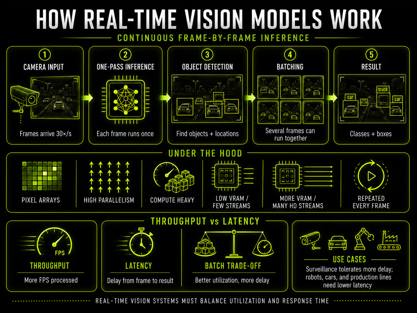
When it comes to real-time object detection, there’s no generation of a specific result. Instead, inference is continuously repeated for each frame. In detectors such as YOLO, everything must be completed in a single pass. To operate in real time, the system receives a frame 30 times per second, passes it through the neural network, identifies objects, and determines where they are located.
From a computational point of view, this workload consists of a large array of pixels, and operations on them can be parallelized extremely well. Therefore, compute becomes the most important metric, while VRAM usage won’t be particularly high. However, this is only true when a single video stream is processed. If you have dozens of high-resolution cameras, the load on compute units increases significantly, and more video memory is required.
To achieve maximum GPU utilization, computations can be performed not on individual images but on a batch of several at once. Still, if some frames have arrived before others, the system will have to wait for them instead of performing the computations. This increases the delay between what the camera sees and the recognition result.
The system, therefore, needs to balance between two parameters: throughput, which means how many frames per second the GPU can process, and latency, or the delay between receiving a frame and producing the result. In ordinary video surveillance, a delay of a couple of hundred milliseconds is perfectly acceptable. However, when dealing with an industrial robot, an autonomous vehicle, or a machine-vision system on a production line, the requirements may be much stricter.
Image Generation

The overwhelming majority of modern neural networks for image generation belong to the class of diffusion models. Despite differences in architecture, all of them rely on the same core principle of repeatedly removing noise.
Basically, the model doesn’t work with pixels directly. It receives images that have been converted into latent space, a compact mathematical representation of the original image. During training, Gaussian noise is gradually added to this latent until the image becomes almost indistinguishable from random noise. At the same time, the neural network learns to predict the direction in which the noisy representation should be changed in order to bring it closer to the original data.
Throughout generation, the process is reversed. The user’s prompt is converted by a text encoder into a set of numerical representations. At the same time, a “canvas” is created (that is, an initial latent space filled with random noise). The neural network then repeatedly processes the latent, removing noise from it step by step while taking the user’s prompt into account. After a certain number of passes, the latent is sent to a VAE decoder, which performs the final conversion into an image.
One factor that significantly affects the workload profile is image resolution. The greater the width and height of the latent, the larger the tensor and, consequently, the greater the number of operations and intermediate activations. Modern models may impose high VRAM requirements, so this parameter will have to be considered first. Bandwidth is also important because the GPU must constantly reread the weights and move tensors between compute units.
Image generation is also demanding in terms of compute performance. As a result, the number of CUDA Cores and Tensor Cores affect generation speed directly. When comparing GPUs, you can use the card’s performance in specific formats, such as FP16, BF16, FP8, and TF32, as a reference.
Video Generation

A video is essentially a sequence of frames, so the basic principle is the same as in standard diffusion generation. The model starts with random noise and transforms it into a meaningful visual signal. However, the task becomes considerably more complex. Across the entire sequence, it’s necessary to preserve the consistency of all objects in the frame, including their positions in space, lighting, perspective, direction of movement, and other visual details. In addition to the two spatial dimensions, a third dimension is introduced: time.
This type of workload is significantly more demanding on the GPU than generating individual images. The architectures of the neural networks used for video generation include object-matching algorithms, spatiotemporal blocks, and frame-position encoders.
Everything still relies on latents. However, the noise-reduction procedure is applied not to individual frames but to the entire sequence, which results in object movements and scene changes being formed consistently. All of this leads to a rapid increase in VRAM consumption. Not only can the model itself easily occupy tens of gigabytes, but also intermediate tensors created during each pass can consume a significant portion of the memory.
As a result, it’s impossible to identify a single dominant characteristic for video generation. VRAM capacity and bandwidth are just as important here as a large number of Tensor and CUDA Cores. To achieve high speeds, servers with multiple GPUs connected by a wide bus such as NVLink are required.
Music Generation

Music generation covers both model types, which is why the right GPU characteristics depend heavily on which one is being used. For instance, models like MusicGen are autoregressive. In them, the user’s prompt is first converted into a conditional context representation, after which the system begins predicting audio tokens one by one, as if it were a language model.
Each subsequent audio token depends on all the previous ones, which means this type of generation will constantly access VRAM during inference. A single second of music consists of numerous tokens from several codebooks, and this requires significantly more iterations than generating a couple of sentences of text. Once the model has generated the required sequence, the decoder reconstructs the final representation from it, like an audio file.
However, there’s also a large separate class of music generators, such as Stable Audio, that use the same principles as diffusion-based image generators. With these models, the system starts with noise and repeatedly passes it through the neural network, removing parts of that noise at each step and gradually refining it into the final signal. Unlike autoregressive models, the neural network here operates on large tensors at once, which allows it to make maximum use of the relevant cores.
Ultimately, the workload profile consists of a large number of parallel matrix operations repeated over multiple steps during which the noise in the latent representation is gradually removed to form the final fragments. In this case, both compute characteristics and VRAM capacity are important factors.
Finally
We have put together a summary table to help you choose an optimal GPU for your workload:
GPU Priorities by Workload
There’s no universal solution that works equally well for every scenario, so the nature of the workload must be taken into account. It can become the decisive factor in building the optimal AI infrastructure.
FAQ
Which GPU specs actually matter for AI?
There are five of them: VRAM, memory bandwidth, compute, interconnect, and the software stack. VRAM determines how much data the card can hold, bandwidth is how fast it can move it, compute represents raw arithmetic, interconnect shows you how efficiently cards can communicate with each other, and the stack is everything above the silicon.
The problem is that no workload relies on all five equally. Trying to rank them in isolation is a wasted effort. You should rank them depending on what you’re actually running.
Is VRAM the most important spec?
No, though it is the number everyone checks first.
VRAM is the priority for chatbots and autoregressive audio models, where the weights and KV cache have somewhere to live. As for image generation, it shares the top spot with compute. When it comes to object detection, though, it barely registers until you start adding cameras.
What is the difference between VRAM and memory bandwidth?
It’s a matter of capacity vs. speed. VRAM determines whether the model loads at all. Bandwidth decides how fast the GPU can pull those weights back out again, along with the KV cache and activations. Having plenty of the first but not enough of the second is the usual reason a card with impressive memory numbers still generates tokens slowly.
Can I compare TFLOPS between two GPUs?
Not without knowing the precision. The same GPU can deliver very different TFLOPS in FP32, FP16, BF16, FP8, and TF32, and vendors quote whatever looks best.
A card marketed on its FP8 figure can sit next to the one quoted in FP32, appear twice as fast on paper, and then end up being roughly equal in your pipeline. Find out what precision your models actually run in, then compare.
What are Tensor Cores?
Tensor Cores are units built for matrix math, which is most of what a neural network does. Though they are less flexible than CUDA Cores, they are much faster at this specific job. They shine on compute-bound work, such as diffusion, video, speech, detection. However, during sequential token generation, they spend a lot of time waiting.
Don't Need Raw GPU Power? You Might Not Have To.
A lot of AI workloads — agent orchestration, chatbot backends, API-based inference — don't touch a GPU at all. They just need a dependable server to run on.
Or see how to deploy an AI agent without local GPU hardware → How to Set Up and Deploy an OpenClaw AI Agent on a VPS


